![]()

Twitter Sentiment Analysis#
By Neuromatch Academy
Content creators: Juan Manuel Rodriguez, Salomey Osei, Gonzalo Uribarri
Production editors: Amita Kapoor, Spiros Chavlis
Welcome to the NLP project template#

Step 1: Questions and goals#
Can we infer emotion from a tweet text?
How words are distributed accross the dataset?
Are words related to one kind of emotion?
Step 2: Literature review#
Step 3: Load and explore the dataset#
# @title Install dependencies
!pip install pandas --quiet
!pip install --upgrade datasets --quiet
?25l   ━━━━━━━━━━━━━━━━━━━━━━━━━━━━━━━━━━━━━━━━ 0.0/491.5 kB ? eta -:--:--
   ━━━━━━━━━━━━━━━━━━━━━━━━━━━━━━━━━━━━━━━━ 491.5/491.5 kB 16.1 MB/s eta 0:00:00
?25h?25l   ━━━━━━━━━━━━━━━━━━━━━━━━━━━━━━━━━━━━━━━━ 0.0/193.6 kB ? eta -:--:--
   ━━━━━━━━━━━━━━━━━━━━━━━━━━━━━━━━━━━━━━━━ 193.6/193.6 kB 17.3 MB/s eta 0:00:00
?25hERROR: pip's dependency resolver does not currently take into account all the packages that are installed. This behaviour is the source of the following dependency conflicts.
gcsfs 2025.3.2 requires fsspec==2025.3.2, but you have fsspec 2025.3.0 which is incompatible.
torch 2.6.0+cu124 requires nvidia-cublas-cu12==12.4.5.8; platform_system == "Linux" and platform_machine == "x86_64", but you have nvidia-cublas-cu12 12.5.3.2 which is incompatible.
torch 2.6.0+cu124 requires nvidia-cuda-cupti-cu12==12.4.127; platform_system == "Linux" and platform_machine == "x86_64", but you have nvidia-cuda-cupti-cu12 12.5.82 which is incompatible.
torch 2.6.0+cu124 requires nvidia-cuda-nvrtc-cu12==12.4.127; platform_system == "Linux" and platform_machine == "x86_64", but you have nvidia-cuda-nvrtc-cu12 12.5.82 which is incompatible.
torch 2.6.0+cu124 requires nvidia-cuda-runtime-cu12==12.4.127; platform_system == "Linux" and platform_machine == "x86_64", but you have nvidia-cuda-runtime-cu12 12.5.82 which is incompatible.
torch 2.6.0+cu124 requires nvidia-cudnn-cu12==9.1.0.70; platform_system == "Linux" and platform_machine == "x86_64", but you have nvidia-cudnn-cu12 9.3.0.75 which is incompatible.
torch 2.6.0+cu124 requires nvidia-cufft-cu12==11.2.1.3; platform_system == "Linux" and platform_machine == "x86_64", but you have nvidia-cufft-cu12 11.2.3.61 which is incompatible.
torch 2.6.0+cu124 requires nvidia-curand-cu12==10.3.5.147; platform_system == "Linux" and platform_machine == "x86_64", but you have nvidia-curand-cu12 10.3.6.82 which is incompatible.
torch 2.6.0+cu124 requires nvidia-cusolver-cu12==11.6.1.9; platform_system == "Linux" and platform_machine == "x86_64", but you have nvidia-cusolver-cu12 11.6.3.83 which is incompatible.
torch 2.6.0+cu124 requires nvidia-cusparse-cu12==12.3.1.170; platform_system == "Linux" and platform_machine == "x86_64", but you have nvidia-cusparse-cu12 12.5.1.3 which is incompatible.
torch 2.6.0+cu124 requires nvidia-nvjitlink-cu12==12.4.127; platform_system == "Linux" and platform_machine == "x86_64", but you have nvidia-nvjitlink-cu12 12.5.82 which is incompatible.
# We import some libraries to load the dataset
import os
import numpy as np
import pandas as pd
import matplotlib.pyplot as plt

from collections import Counter
from tqdm.notebook import tqdm

import torch
import torch.nn as nn
import torch.optim as optim
import torch.nn.functional as F
from torch.utils.data import TensorDataset, DataLoader
import spacy

import re
from sklearn.utils import shuffle
from sklearn.metrics import classification_report
from sklearn.linear_model import LogisticRegression
from sklearn.model_selection import train_test_split
from sklearn.feature_extraction.text import CountVectorizer
Helper functions#
_patterns = [r"\'", r"\"", r"\.", r"<br \/>", r",", r"\(", r"\)", r"\!", r"\?", r"\;", r"\:", r"\s+"]

_replacements = [" '  ", "", " . ", " ", " , ", " ( ", " ) ", " ! ", " ? ", " ", " ", " "]

_patterns_dict = list((re.compile(p), r) for p, r in zip(_patterns, _replacements))

def _basic_english_normalize(line):
    r"""
    Basic normalization for a line of text.
    Normalization includes
    - lowercasing
    - complete some basic text normalization for English words as follows:
        add spaces before and after '\''
        remove '\"',
        add spaces before and after '.'
        replace '<br \/>'with single space
        add spaces before and after ','
        add spaces before and after '('
        add spaces before and after ')'
        add spaces before and after '!'
        add spaces before and after '?'
        replace ';' with single space
        replace ':' with single space
        replace multiple spaces with single space

    Returns a list of tokens after splitting on whitespace.
    """

    line = line.lower()
    for pattern_re, replaced_str in _patterns_dict:
        line = pattern_re.sub(replaced_str, line)
    return line.split()


def get_tokenizer(tokenizer, language='en'):
    r"""
    Generate tokenizer function for a string sentence.

    Arguments:
        tokenizer: the name of tokenizer function. If None, it returns split()
            function, which splits the string sentence by space.
            If basic_english, it returns _basic_english_normalize() function,
            which normalize the string first and split by space. If a callable
            function, it will return the function. If a tokenizer library
            (e.g. spacy, moses, toktok, revtok, subword), it returns the
            corresponding library.
        language: Default en

    Examples:
        >>> import torchtext
        >>> from torchtext.data import get_tokenizer
        >>> tokenizer = get_tokenizer("basic_english")
        >>> tokens = tokenizer("You can now install TorchText using pip!")
        >>> tokens
        >>> ['you', 'can', 'now', 'install', 'torchtext', 'using', 'pip', '!']

    """

    # default tokenizer is string.split(), added as a module function for serialization


    if tokenizer == "basic_english":
        if language != 'en':
            raise ValueError("Basic normalization is only available for Enlish(en)")
        return _basic_english_normalize

    # simply return if a function is passed
    if callable(tokenizer):
        return tokenizer

    if tokenizer == "spacy":
        try:
            import spacy
            spacy = spacy.load(language)
            return partial(_spacy_tokenize, spacy=spacy)
        except ImportError:
            print("Please install SpaCy. "
                  "See the docs at https://spacy.io for more information.")
            raise
        except AttributeError:
            print("Please install SpaCy and the SpaCy {} tokenizer. "
                  "See the docs at https://spacy.io for more "
                  "information.".format(language))
            raise
    elif tokenizer == "moses":
        try:
            from sacremoses import MosesTokenizer
            moses_tokenizer = MosesTokenizer()
            return moses_tokenizer.tokenize
        except ImportError:
            print("Please install SacreMoses. "
                  "See the docs at https://github.com/alvations/sacremoses "
                  "for more information.")
            raise
    elif tokenizer == "toktok":
        try:
            from nltk.tokenize.toktok import ToktokTokenizer
            toktok = ToktokTokenizer()
            return toktok.tokenize
        except ImportError:
            print("Please install NLTK. "
                  "See the docs at https://nltk.org  for more information.")
            raise
    elif tokenizer == 'revtok':
        try:
            import revtok
            return revtok.tokenize
        except ImportError:
            print("Please install revtok.")
            raise
    elif tokenizer == 'subword':
        try:
            import revtok
            return partial(revtok.tokenize, decap=True)
        except ImportError:
            print("Please install revtok.")
            raise
    raise ValueError("Requested tokenizer {}, valid choices are a "
                     "callable that takes a single string as input, "
                     "\"revtok\" for the revtok reversible tokenizer, "
                     "\"subword\" for the revtok caps-aware tokenizer, "
                     "\"spacy\" for the SpaCy English tokenizer, or "
                     "\"moses\" for the NLTK port of the Moses tokenization "
                     "script.".format(tokenizer))
Dataset#
You can find the dataset we are going to use in this website.
from datasets import load_dataset
dataset = load_dataset("stanfordnlp/sentiment140", trust_remote_code=True)
# We load the dataset
train_data = dataset["train"]
df = pd.DataFrame(train_data)
df = df.rename(columns={'sentiment': 'polarity'})
df = df[['polarity', 'user', 'date', 'query', 'user', 'text']]
df.head()
DATASET_SIZE=10000

# Limit the dataset size
df = df[:DATASET_SIZE]

# Show the first few rows
df.head()
| polarity | user | date | query | user | text | |
|---|---|---|---|---|---|---|
| 0 | 0 | _TheSpecialOne_ | Mon Apr 06 22:19:45 PDT 2009 | NO_QUERY | _TheSpecialOne_ | @switchfoot http://twitpic.com/2y1zl - Awww, t... |
| 1 | 0 | scotthamilton | Mon Apr 06 22:19:49 PDT 2009 | NO_QUERY | scotthamilton | is upset that he can't update his Facebook by ... |
| 2 | 0 | mattycus | Mon Apr 06 22:19:53 PDT 2009 | NO_QUERY | mattycus | @Kenichan I dived many times for the ball. Man... |
| 3 | 0 | ElleCTF | Mon Apr 06 22:19:57 PDT 2009 | NO_QUERY | ElleCTF | my whole body feels itchy and like its on fire |
| 4 | 0 | Karoli | Mon Apr 06 22:19:57 PDT 2009 | NO_QUERY | Karoli | @nationwideclass no, it's not behaving at all.... |
For this project we will use only the text and the polarity of the tweet. Notice that polarity is 0 for negative tweets and 4 for positive tweet.
X = df.text.values

# Changes values from [0,4] to [0,1]
y = (df.polarity.values > 1).astype(int)


# Split the data into train and test
x_train_text, x_test_text, y_train, y_test = train_test_split(X, y, test_size=0.2, random_state=42,stratify=y)
The first thing we have to do before working on the models is to familiarize ourselves with the dataset. This is called Exploratory Data Analisys (EDA).
for s, l in zip(x_train_text[:5], y_train[:5]):
  print('{}: {}'.format(l, s))
0: equinux.com just crashed safari tks you!
0: tierd  whats pt swagger mean.. i love the sound of it
0: @EstelleDarlings Honestly, you can only speak to urself because no 1 cares @the airport. Someone will always direct u 2 the next person
0: Site load rising again. Increased my capacity but it's going up still
0: @heidimontag just got done watching the hills! loved it! excited for the next episode! and im sad this is the last season!
An interesting thing to analyze is the Word Distribution. In order to count the occurrences of each word, we should tokenize the sentences first.
tokenizer = get_tokenizer("basic_english")

print('Before Tokenize: ', x_train_text[1])
print('After Tokenize: ', tokenizer(x_train_text[1]))
Before Tokenize:  tierd  whats pt swagger mean.. i love the sound of it
After Tokenize:  ['tierd', 'whats', 'pt', 'swagger', 'mean', '.', '.', 'i', 'love', 'the', 'sound', 'of', 'it']
x_train_token = [tokenizer(s) for s in tqdm(x_train_text)]
x_test_token = [tokenizer(s) for s in tqdm(x_test_text)]
We can count the words occurences and see how many different words are present in our dataset.
words = Counter()
for s in x_train_token:
  for w in s:
    words[w] += 1

sorted_words = list(words.keys())
sorted_words.sort(key=lambda w: words[w], reverse=True)
print(f"Number of different Tokens in our Dataset: {len(sorted_words)}")
print(sorted_words[:100])
Number of different Tokens in our Dataset: 14815
['.', 'i', "'", '!', 'to', 'the', ',', 'a', 'my', 'it', 'and', 'is', '?', 't', 'in', 'for', 'of', 'you', 's', 'but', 'me', 'on', 'that', 'have', 'not', 'so', 'm', 'at', 'just', 'this', 'be', 'was', 'work', 'up', 'with', 'now', 'no', 'can', 'get', 'out', 'go', 'all', 'today', 'day', 'too', 'like', 'do', 'don', 'still', 'going', '-', 'got', 'are', 'back', 'am', 'really', 'time', 'what', 'from', 'about', 'has', 'had', 'one', 'good', 'its', 'they', 'want', 'im', 'sad', 'we', 'why', 'need', 'home', 'http', 'sleep', 'your', 'know', 'night', 'when', 'there', 'some', 'will', 'more', 'oh', 'been', 'lol', 'last', 'feel', 'sick', 'miss', '2', 'morning', 'much', 'again', 'off', 'sorry', 'as', 'think', 'wish', 'an']
Now we can plot their distribution.
count_occurences = sum(words.values())

accumulated = 0
counter = 0

while accumulated < count_occurences * 0.8:
  accumulated += words[sorted_words[counter]]
  counter += 1

print(f"The {counter * 100 / len(words)}% most common words "
      f"account for the {accumulated * 100 / count_occurences}% of the occurrences")
The 5.190685116436044% most common words account for the 80.00869187309866% of the occurrences
plt.bar(range(100), [words[w] for w in sorted_words[:100]])
plt.show()
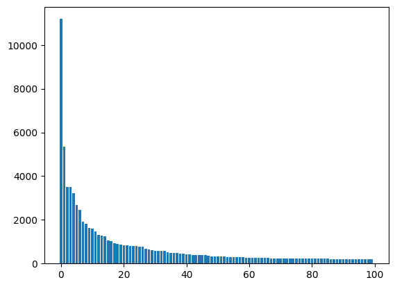
It is very common to find this kind of distribution when analyzing corpus of text. This is referred to as the zipf’s law.
Usually the number of words in the dictionary will be very large.
Here are some thing we can do to reduce that number:
Remove puntuation.
Remove stop-words.
Steaming.
Remove very uncommon words (the words that appears in fewer than N occations).
Nothing: we can use a pretrain model that handles this kind of situations.
We used one of the simplest tokenizers availables. This tokenizer does not take into account many quirks of the language. Moreover, diferent languages have different quirks, so there is no “universal” tokenizers. There are many libraries that have “better” tokenizers:
Spacy: it can be accessed using:
get_tokenizer("spacy"). Spacy supports a wide range of languages.Huggingface: it has many tokenizers for different laguages. Doc
NLTK: it provides several tokenizers. One of them can be accessed using:
get_tokenizer("toktok")
Step 4: choose toolkit#
Our goal is to train a model capable of estimating the sentiment of a tweet (positive or negative) by reading its content. To that end we will try 2 different approaches:
A logistic regression using sklearn. NOTE: it can probaly work better than an SVM model.
A simple Embedding + RNN.
Logistic regression#
We will represent our senteces using binary vectorization. This means that our data would be represented as a matrix of instances by word with a one if the word is in the instance, and zero otherwise. Sklean vectorizers can also do things such as stop-word removal and puntuation removal, you can read more about in the documentation.
vectorizer = CountVectorizer(binary=True)
x_train_cv = vectorizer.fit_transform(x_train_text)
x_test_cv = vectorizer.transform(x_test_text)
print('Before Vectorize: ', x_train_text[3])
Before Vectorize: Site load rising again. Increased my capacity but it's going up still
# Notice that the matriz is sparse
print('After Vectorize: ')
print(x_train_cv[3])
After Vectorize:
<Compressed Sparse Row sparse matrix of dtype 'int64'
	with 12 stored elements and shape (1, 14159)>
  Coords	Values
  (0, 6377)	1
  (0, 11286)	1
  (0, 7410)	1
  (0, 10478)	1
  (0, 655)	1
  (0, 6190)	1
  (0, 8422)	1
  (0, 2199)	1
  (0, 2086)	1
  (0, 5251)	1
  (0, 13169)	1
  (0, 11819)	1
Now we can train our model. You can check the documentation of this logistic regressor here.
model = LogisticRegression(solver='saga')
model.fit(x_train_cv, y_train)
---------------------------------------------------------------------------
ValueError                                Traceback (most recent call last)
/tmp/ipython-input-23-2773398188.py in <cell line: 0>()
      1 model = LogisticRegression(solver='saga')
----> 2 model.fit(x_train_cv, y_train)

/usr/local/lib/python3.11/dist-packages/sklearn/base.py in wrapper(estimator, *args, **kwargs)
   1387                 )
   1388             ):
-> 1389                 return fit_method(estimator, *args, **kwargs)
   1390
   1391         return wrapper

/usr/local/lib/python3.11/dist-packages/sklearn/linear_model/_logistic.py in fit(self, X, y, sample_weight)
   1299         classes_ = self.classes_
   1300         if n_classes < 2:
-> 1301             raise ValueError(
   1302                 "This solver needs samples of at least 2 classes"
   1303                 " in the data, but the data contains only one"

ValueError: This solver needs samples of at least 2 classes in the data, but the data contains only one class: np.int64(0)
y_pred = model.predict(x_test_cv)

print(classification_report(y_test, y_pred))
Explainable AI#
The best thing about logistic regresion is that it is simple, and we can get some explanations.
print(model.coef_.shape)
print(len(vectorizer.vocabulary_))

words_sk = list(vectorizer.vocabulary_.keys())
words_sk.sort(key=lambda w: model.coef_[0, vectorizer.vocabulary_[w]])
---------------------------------------------------------------------------
AttributeError                            Traceback (most recent call last)
/tmp/ipython-input-24-3113506201.py in <cell line: 0>()
----> 1 print(model.coef_.shape)
      2 print(len(vectorizer.vocabulary_))
      3
      4 words_sk = list(vectorizer.vocabulary_.keys())
      5 words_sk.sort(key=lambda w: model.coef_[0, vectorizer.vocabulary_[w]])

AttributeError: 'LogisticRegression' object has no attribute 'coef_'
for w in words_sk[:20]:
  print('{}: {}'.format(w, model.coef_[0, vectorizer.vocabulary_[w]]))
for w in reversed(words_sk[-20:]):
  print('{}: {}'.format(w, model.coef_[0, vectorizer.vocabulary_[w]]))
What does this mean?
Remember the model.coef_ is the \(W\) in:
where the label 1 is a positive tweet and the label 0 is a negative tweet.
Recurrent Neural Network with Pytorch#
In the previous section we use a Bag-Of-Words approach to represent each of the tweets. That meas that we only consider how many times each of the words appear in each of the tweets, we didnt take into account the order of the words. But we know that the word order is very important and carries relevant information.
In this section we will solve the same task, but this time we will implement a Recurrent Neural Network (RNN) instead of using a simple Logistic Regression.Unlike feedforward neural networks, RNNs have cyclic connections making them powerful for modeling sequences.
Let’s start by importing the relevant libraries.
def set_device():
  device = "cuda" if torch.cuda.is_available() else "cpu"
  if device != "cuda":
    print("WARNING: For this notebook to perform best, "
          "if possible, in the menu under `Runtime` -> "
          "`Change runtime type.`  select `GPU` ")
  else:
    print("GPU is enabled in this notebook.")

  return device
# Set the device (check if gpu is available)
device = set_device()
GPU is enabled in this notebook.
First we will create a Dictionary (word_to_idx). This dictionary will map each Token (usually words) to an index (an integer number). We want to limit our dictionary to a certain number of tokens (num_words_dict), so we will include in our ditionary those with more occurrences.
# From previous section, we have a list with the most used tokens
sorted_words[:10]
['.', 'i', "'", '!', 'to', 'the', ',', 'a', 'my', 'it']
Let’s select only the most used.
num_words_dict = 30000
# We reserve two numbers for special tokens.
most_used_words = sorted_words[:num_words_dict-2]
We will add two extra Tokens to the dictionary, one for words outside the dictionary ('UNK') and one for padding the sequences ('PAD').
# dictionary to go from words to idx
word_to_idx = {}
# dictionary to go from idx to words (just in case)
idx_to_word = {}


# We include the special tokens first
PAD_token = 0
UNK_token = 1

word_to_idx['PAD'] = PAD_token
word_to_idx['UNK'] = UNK_token

idx_to_word[PAD_token] = 'PAD'
idx_to_word[UNK_token] = 'UNK'

# We popullate our dictionaries with the most used words
for num,word in enumerate(most_used_words):
  word_to_idx[word] = num + 2
  idx_to_word[num+2] = word
Our goal now is to transform each tweet from a sequence of tokens to a sequence of indexes. These sequences of indexes will be the input to our pytorch model.
# A function to convert list of tokens to list of indexes
def tokens_to_idx(sentences_tokens,word_to_idx):
  sentences_idx = []
  for sent in sentences_tokens:
    sent_idx = []
    for word in sent:
      if word in word_to_idx:
        sent_idx.append(word_to_idx[word])
      else:
        sent_idx.append(word_to_idx['UNK'])
    sentences_idx.append(sent_idx)
  return sentences_idx
x_train_idx = tokens_to_idx(x_train_token,word_to_idx)
x_test_idx = tokens_to_idx(x_test_token,word_to_idx)
some_number = 1
print('Before converting: ', x_train_token[some_number])
print('After converting: ', x_train_idx[some_number])
Before converting:  ['tierd', 'whats', 'pt', 'swagger', 'mean', '.', '.', 'i', 'love', 'the', 'sound', 'of', 'it']
After converting:  [4880, 801, 2396, 4881, 391, 2, 2, 3, 120, 7, 631, 18, 11]
We need all the sequences to have the same length. To select an adequate sequence length, let’s explore some statistics about the length of the tweets:
tweet_lens = np.asarray([len(sentence) for sentence in x_train_idx])
print('Max tweet word length: ',tweet_lens.max())
print('Mean tweet word length: ',np.median(tweet_lens))
print('99% percent under: ',np.quantile(tweet_lens,0.99))
Max tweet word length:  62
Mean tweet word length:  16.0
99% percent under:  37.0
We cut the sequences which are larger than our chosen maximum length (max_lenght) and fill with zeros the ones that are shorter.
 # We choose the max length
 max_length = 40

# A function to make all the sequence have the same lenght
# Note that the output is a Numpy matrix
 def padding(sentences, seq_len):
  features = np.zeros((len(sentences), seq_len),dtype=int)
  for ii, tweet in enumerate(sentences):
    len_tweet = len(tweet)
    if len_tweet != 0:
      if len_tweet <= seq_len:
        # If its shorter, we fill with zeros (the padding Token index)
        features[ii, -len(tweet):] = np.array(tweet)[:seq_len]
      if len_tweet > seq_len:
        # If its larger, we take the last 'seq_len' indexes
        features[ii, :] = np.array(tweet)[-seq_len:]
  return features
# We convert our list of tokens into a numpy matrix
# where all instances have the same lenght
x_train_pad = padding(x_train_idx,max_length)
x_test_pad = padding(x_test_idx,max_length)

# We convert our target list a numpy matrix
y_train_np = np.asarray(y_train)
y_test_np = np.asarray(y_test)
some_number = 2
print('Before padding: ', x_train_idx[some_number])
print('After padding: ', x_train_pad[some_number])
Before padding:  [4882, 1701, 8, 19, 39, 103, 765, 6, 3175, 196, 38, 249, 4883, 4884, 976, 2, 234, 83, 235, 1980, 123, 92, 7, 236, 911]
After padding:  [   0    0    0    0    0    0    0    0    0    0    0    0    0    0
    0 4882 1701    8   19   39  103  765    6 3175  196   38  249 4883
 4884  976    2  234   83  235 1980  123   92    7  236  911]
Now, let’s convert the data to pytorch format.
# create Tensor datasets
train_data = TensorDataset(torch.from_numpy(x_train_pad), torch.from_numpy(y_train_np))
valid_data = TensorDataset(torch.from_numpy(x_test_pad), torch.from_numpy(y_test_np))

# Batch size (this is an important hyperparameter)
batch_size = 100

# dataloaders
# make sure to SHUFFLE your data
train_loader = DataLoader(train_data, shuffle=True, batch_size=batch_size,drop_last = True)
valid_loader = DataLoader(valid_data, shuffle=True, batch_size=batch_size,drop_last = True)
Each batch of data in our traning proccess will have the folllowing format:
# Obtain one batch of training data
dataiter = iter(train_loader)
sample_x, sample_y = dataiter.__next__()

print('Sample input size: ', sample_x.size()) # batch_size, seq_length
print('Sample input: \n', sample_x)
print('Sample input: \n', sample_y)
Sample input size:  torch.Size([100, 40])
Sample input:
 tensor([[    0,     0,     0,  ...,   303,   856, 14628],
        [    0,     0,     0,  ...,  3102,    33,   111],
        [    0,     0,     0,  ..., 10228,    22,    46],
        ...,
        [    0,     0,     0,  ...,     6,    42,   128],
        [    0,     0,     0,  ...,   350,  1305,  4700],
        [    0,     0,     0,  ...,  7050,  7051,  7052]])
Sample input:
 tensor([0, 0, 0, 0, 0, 0, 0, 0, 0, 0, 0, 0, 0, 0, 0, 0, 0, 0, 0, 0, 0, 0, 0, 0,
        0, 0, 0, 0, 0, 0, 0, 0, 0, 0, 0, 0, 0, 0, 0, 0, 0, 0, 0, 0, 0, 0, 0, 0,
        0, 0, 0, 0, 0, 0, 0, 0, 0, 0, 0, 0, 0, 0, 0, 0, 0, 0, 0, 0, 0, 0, 0, 0,
        0, 0, 0, 0, 0, 0, 0, 0, 0, 0, 0, 0, 0, 0, 0, 0, 0, 0, 0, 0, 0, 0, 0, 0,
        0, 0, 0, 0])
Now, we will define the SentimentRNN class. Most of the model’s class will be familiar to you, but there are two important layers we would like you to pay attention to:
Embedding Layer
This layer is like a linear layer, but it makes it posible to use a sequence of inedexes as inputs (instead of a sequence of one-hot-encoded vectors). During training, the Embedding layer learns a linear transformation from the space of words (a vector space of dimension
num_words_dict) into the a new, smaller, vector space of dimensionembedding_dim. We suggest you to read this thread and the pytorch documentation if you want to learn more about this particular kind of layers.
LSTM layer
This is one of the most used class of Recurrent Neural Networks. In Pytorch we can add several stacked layers in just one line of code. In our case, the number of layers added are decided with the parameter
no_layers. If you want to learn more about LSTMs we strongly recommend you this Colahs thread about them.
class SentimentRNN(nn.Module):
  def __init__(self,no_layers,vocab_size,hidden_dim,embedding_dim,drop_prob=0.1):
    super(SentimentRNN,self).__init__()

    self.output_dim = output_dim
    self.hidden_dim = hidden_dim
    self.no_layers = no_layers
    self.vocab_size = vocab_size
    self.drop_prob = drop_prob

    # Embedding Layer
    self.embedding = nn.Embedding(vocab_size, embedding_dim)

    # LSTM Layers
    self.lstm = nn.LSTM(input_size=embedding_dim,hidden_size=self.hidden_dim,
                        num_layers=no_layers, batch_first=True,
                        dropout=self.drop_prob)

    # Dropout layer
    self.dropout = nn.Dropout(drop_prob)

    # Linear and Sigmoid layer
    self.fc = nn.Linear(self.hidden_dim, output_dim)
    self.sig = nn.Sigmoid()

  def forward(self,x,hidden):
    batch_size = x.size(0)

    # Embedding out
    embeds = self.embedding(x)
    #Shape: [batch_size x max_length x embedding_dim]

    # LSTM out
    lstm_out, hidden = self.lstm(embeds, hidden)
    # Shape: [batch_size x max_length x hidden_dim]

    # Select the activation of the last Hidden Layer
    lstm_out = lstm_out[:,-1,:].contiguous()
    # Shape: [batch_size x hidden_dim]

    ## You can instead average the activations across all the times
    # lstm_out = torch.mean(lstm_out, 1).contiguous()

    # Dropout and Fully connected layer
    out = self.dropout(lstm_out)
    out = self.fc(out)

    # Sigmoid function
    sig_out = self.sig(out)

    # return last sigmoid output and hidden state
    return sig_out, hidden

  def init_hidden(self, batch_size):
    ''' Initializes hidden state '''
    # Create two new tensors with sizes n_layers x batch_size x hidden_dim,
    # initialized to zero, for hidden state and cell state of LSTM
    h0 = torch.zeros((self.no_layers,batch_size,self.hidden_dim)).to(device)
    c0 = torch.zeros((self.no_layers,batch_size,self.hidden_dim)).to(device)
    hidden = (h0,c0)
    return hidden
We choose the parameters of the model.
# Parameters of our network

# Size of our vocabulary
vocab_size = num_words_dict

# Embedding dimension
embedding_dim = 32

# Number of stacked LSTM layers
no_layers = 2

# Dimension of the hidden layer in LSTMs
hidden_dim = 64

# Dropout parameter for regularization
output_dim = 1

# Dropout parameter for regularization
drop_prob = 0.25
# Let's define our model
model = SentimentRNN(no_layers, vocab_size, hidden_dim,
                     embedding_dim, drop_prob=drop_prob)
# Moving to gpu
model.to(device)
print(model)
SentimentRNN(
  (embedding): Embedding(30000, 32)
  (lstm): LSTM(32, 64, num_layers=2, batch_first=True, dropout=0.25)
  (dropout): Dropout(p=0.25, inplace=False)
  (fc): Linear(in_features=64, out_features=1, bias=True)
  (sig): Sigmoid()
)
# How many trainable parameters does our model have?
model_parameters = filter(lambda p: p.requires_grad, model.parameters())
params = sum([np.prod(p.size()) for p in model_parameters])
print('Total Number of parameters: ',params)
Total Number of parameters: 1018433
We choose the losses and the optimizer for the training procces.
# loss and optimization functions
lr = 0.001

# Binary crossentropy is a good loss function for a binary classification problem
criterion = nn.BCELoss()

# We choose an Adam optimizer
optimizer = torch.optim.Adam(model.parameters(), lr=lr)

# function to predict accuracy
def acc(pred,label):
  pred = torch.round(pred.squeeze())
  return torch.sum(pred == label.squeeze()).item()
We are ready to train our model.
# Number of training Epochs
epochs = 5

# Maximum absolute value accepted for the gradeint
clip = 5

# Initial Loss value (assumed big)
valid_loss_min = np.inf

# Lists to follow the evolution of the loss and accuracy
epoch_tr_loss,epoch_vl_loss = [],[]
epoch_tr_acc,epoch_vl_acc = [],[]

# Train for a number of Epochs
for epoch in range(epochs):
  train_losses = []
  train_acc = 0.0
  model.train()

  for inputs, labels in train_loader:

    # Initialize hidden state
    h = model.init_hidden(batch_size)
    # Creating new variables for the hidden state
    h = tuple([each.data.to(device) for each in h])

    # Move batch inputs and labels to gpu
    inputs, labels = inputs.to(device), labels.to(device)

    # Set gradient to zero
    model.zero_grad()

    # Compute model output
    output,h = model(inputs,h)

    # Calculate the loss and perform backprop
    loss = criterion(output.squeeze(), labels.float())
    loss.backward()
    train_losses.append(loss.item())

    # calculating accuracy
    accuracy = acc(output,labels)
    train_acc += accuracy

    #`clip_grad_norm` helps prevent the exploding gradient problem in RNNs / LSTMs.
    nn.utils.clip_grad_norm_(model.parameters(), clip)
    optimizer.step()


  # Evaluate on the validation set for this epoch
  val_losses = []
  val_acc = 0.0
  model.eval()
  for inputs, labels in valid_loader:

    # Initialize hidden state
    val_h = model.init_hidden(batch_size)
    val_h = tuple([each.data.to(device) for each in val_h])

    # Move batch inputs and labels to gpu
    inputs, labels = inputs.to(device), labels.to(device)

    # Compute model output
    output, val_h = model(inputs, val_h)

    # Compute Loss
    val_loss = criterion(output.squeeze(), labels.float())

    val_losses.append(val_loss.item())

    accuracy = acc(output,labels)
    val_acc += accuracy

  epoch_train_loss = np.mean(train_losses)
  epoch_val_loss = np.mean(val_losses)
  epoch_train_acc = train_acc/len(train_loader.dataset)
  epoch_val_acc = val_acc/len(valid_loader.dataset)
  epoch_tr_loss.append(epoch_train_loss)
  epoch_vl_loss.append(epoch_val_loss)
  epoch_tr_acc.append(epoch_train_acc)
  epoch_vl_acc.append(epoch_val_acc)
  print(f'Epoch {epoch+1}')
  print(f'train_loss : {epoch_train_loss} val_loss : {epoch_val_loss}')
  print(f'train_accuracy : {epoch_train_acc*100} val_accuracy : {epoch_val_acc*100}')
  if epoch_val_loss <= valid_loss_min:
    print('Validation loss decreased ({:.6f} --> {:.6f}).  Saving model ...'.format(valid_loss_min,epoch_val_loss))
    # torch.save(model.state_dict(), '../working/state_dict.pt')
    valid_loss_min = epoch_val_loss
  print(25*'==')
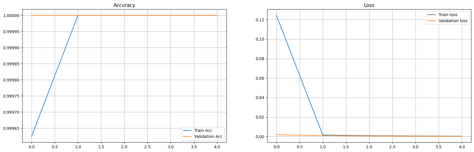
Epoch 1
train_loss : 0.12438914714439306 val_loss : 0.0018169824266806244
train_accuracy : 99.9625 val_accuracy : 100.0
Validation loss decreased (inf --> 0.001817).  Saving model ...
==================================================
Epoch 2
train_loss : 0.0015338497134507634 val_loss : 0.0009810010727960617
train_accuracy : 100.0 val_accuracy : 100.0
Validation loss decreased (0.001817 --> 0.000981).  Saving model ...
==================================================
Epoch 3
train_loss : 0.0009141735477896873 val_loss : 0.0006214575550984591
train_accuracy : 100.0 val_accuracy : 100.0
Validation loss decreased (0.000981 --> 0.000621).  Saving model ...
==================================================
Epoch 4
train_loss : 0.0006109651429142104 val_loss : 0.000429066653305199
train_accuracy : 100.0 val_accuracy : 100.0
Validation loss decreased (0.000621 --> 0.000429).  Saving model ...
==================================================
Epoch 5
train_loss : 0.00044310156408755574 val_loss : 0.00031149635469773784
train_accuracy : 100.0 val_accuracy : 100.0
Validation loss decreased (0.000429 --> 0.000311).  Saving model ...
==================================================
fig = plt.figure(figsize = (20, 6))
plt.subplot(1, 2, 1)
plt.plot(epoch_tr_acc, label='Train Acc')
plt.plot(epoch_vl_acc, label='Validation Acc')
plt.title("Accuracy")
plt.legend()
plt.grid()

plt.subplot(1, 2, 2)
plt.plot(epoch_tr_loss, label='Train loss')
plt.plot(epoch_vl_loss, label='Validation loss')
plt.title("Loss")
plt.legend()
plt.grid()

plt.show()
What’s Next?#
You can use this project template as a starting point to think about your own project. There are a lot of ways to continue, here we share with you some ideas you migth find useful:
Work on the Preproccesing. We used a very rudimentary way to tokenize tweets. But there are better ways to preprocess the data. Can you think of a suitable way to preprocess the data for this particular task? How does the performance of the model change when the data is processed correctly?
Work on the Model. The RNN model proposed in this notebook is not optimized at all. You can work on finding a better architecture or better hyperparamenters. May be using bidirectonal LSTMs or increasing the number of stacked layers can improve the performance, feel free to try different approaches.
Work on the Embedding. Our model learnt an embedding during the training on this Twitter corpus for a particular task. You can explore the representation of different words in this learned embedding. Also, you can try using different word embeddings. You can train them on this corpus or you can use an embedding trained on another corpus of data. How does the change of the embedding affect the model performance?
Try sentiment analysis on another dataset. There are lots of available dataset to work with, we can help you find one that is interesting to you. Do you belive that a sentiment analysis model trained on some corpus (Twitter dataset) will perform well on another type of data (for example, youtube comments)?